Signal with a n-th order response time
ClassName
“Response_Time”
Icon
`
“data_treatment”
Categories
all
Description
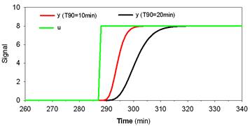
The model describes the dynamic behaviour of a signal that is subjected to input dynamics (cf. figure).
The dynamic behaviour of the response time is modelled through a series of Laplace transfer functions (i.e. creating an n-th order linear system composed of n first order differential equations) as in the following equation:
![]()
where:
· Tau denotes the time constant
· n ranges from 1 to 8 and denotes the order of the response time (i.e. the number of transfer functions in series).
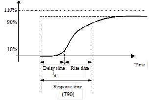
For convenience, the parameter Tau is expressed as a function of T90, which is defined as the overall time to reach (and not to leave) a 90-110% band of the final value of the step response (as shown in figure; adapted from Rieger et al., 2003).
The T90 / Tau relationship was numerically calculated (more information in Alex et al., 2009) and the results are show in the following table.
|
n |
1 |
2 |
3 |
4 |
5 |
6 |
7 |
8 |
|
Tau90/Tau |
2.3247 |
3.89 |
5.3336 |
6.6902 |
8.0031 |
9.2680 |
10.5357 |
11.7724 |
Remark: the T90 value needs to be greater than the minimum step size of the solver.
Parameters
|
Name |
Description |
Value |
Units |
|
n |
Order for the response time (2-8) |
2 |
n/a |
|
T90 |
Response time |
0.00694 |
d |
State Variables
|
Name |
Description |
Units |
|
Tau |
Time constant |
d |
Derived State Variables
None
Interface Variables
|
Name |
Terminal |
Description |
Value |
Units |
|
u |
in_1 |
Signal input |
--- |
--- |
|
y_M |
out_1 |
Signal output |
--- |
--- |
References
Rieger L., Alex J., Winkler S., Boehler M., Thomann M. and Siegrist H. (2003). Progress in sensor technology - progress in process control? Part I: Sensor property investigation and classification. Water Sci. Technol., 47(2), 103-112.
![]()